

Press F12 at any time to show the Graphing & List Window, or select Graphing & List from the Window main menu.
The Graphing and Professional* editions of DreamCalc allow you to graph functions, plot data and edit lists. DreamCalc can graph two functions simultaneously and show a range of charts, including histograms, bar charts, polar plots and regression fits. You can also use this window to perform numerical calculus and statistical calculations.
As shown below, the window comprises a two page layout with a graph view and a list data page. The list page provides a spreadsheet style interface for inputting statistical and X-Y data values for use in both generating charts and performing statistical calculations.
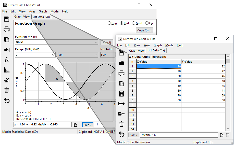
DreamCalc Graphing & List Window
The following chart types are supported:
*Professional Edition Only.
To graph a function, simply select Function Graph from the window's Graph menu and type in the function expression using "x" as the independent variable. Specify the x-value range and click Enter.
See Graphing a Function for further information.
To display statistical data, first put the calculator into the Statistical Data (SD) mode, and then select a suitable chart, i.e. a histogram, from the Graph→Statistical Charts menu.
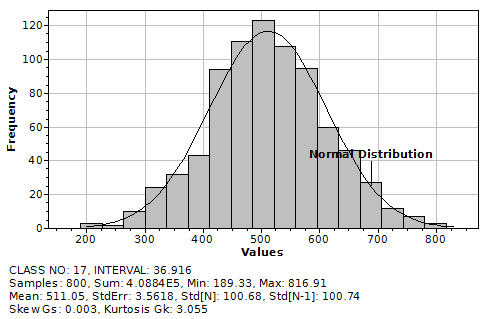
Further information is available for Statistical Charts.
To plot X-Y data, first put the calculator into a suitable X-Y data mode from the Window's Mode menu. For example, click Mode→Linear Regression (X-Y). Next click the list page tab and enter your X-Y data (you may copy and paste from a spreadsheet application or import a file).
Then select a suitable X-Y plot from the Graph menu, i.e. Graph→X-Y Data Plots→Scatter Points.
Additionally, you can elect to show (or hide) the line of best fit by toggling the Show Regression Fit menu option under X-Y Data Plots.
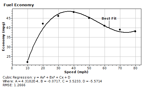
The example above shows an X-Y scatter plot with a cubic regression fit. You can also toggle the statistical information shown beneath the plot by selecting View→Show Footer.
An X-Y style chart can be shown with logarithmic axes, or converted to polar form. Use the Axes menu to select from the available options. You may select logarithmic scales for x and y axes independently. See also Polar Plots for further information.
You can perform chart zooming by simply dragging a rectangle over an area of interest with the mouse. To unzoom, click the [UNZOOM] label which will appear at the bottom right of the chart, or select View→Unzoom.
You can use your mouse to trace along a plotted curve — a circular marker will automatically follow the path of the plot. The coordinates of the plot cursor will be shown in the lower left of the window (see below).
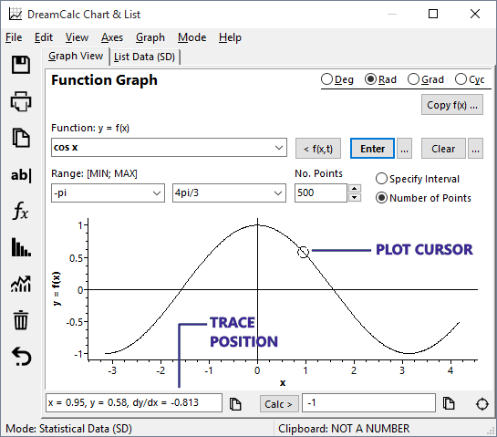
Plot Cursor
Values are shown to the precision allowed by the size of the graphing window. If two plots are visible, the trace marker will follow the plot nearest to the mouse cursor.
You can get a "fix" of the current cursor position at any time by single clicking on the chart at the desired location.
Try this...
You will now see the coordinates, along with the gradient, stored in the position box under the chart. You can click the copy button to the right of the box to copy the text to the clipboard.
You can calculate numerical integrals, derivatives (dy/dx) and x-axis intercepts with any X-Y plot. In addition, you can find intersection points of dual function plots.
See the page on numerical calculus for more information.
A chart can be saved as one of several commonly used image formats from the window's File menu.
Perhaps the easiest method of export, however, is to simply copy the chart into the clipboard using the Edit menu. Two copy options are available: copy as metafile or bitmap. The metafile format is ideal for pasting into documents because it is vector based and can be resized without loss of resolution. However, there may be instances where only a bitmap is compatible.
See also: Graphing a Function, Graphing Examples, Standard Deviation Charts, Numerical Calculus.