

DreamCalc supports statistical calculations with list data.
DreamCalc maintains two independent data lists for use in statistical calculations — namely an X-Y list and a Statistical Data (SD) list. The X-Y list is used in regression analysis, while the SD list holds values with corresponding frequencies, or weights, for use in statistical data calculations.
The calculator's statistical mode designates which data list is in current use. You can switch statistical mode instantly from either the Modes→Statistics menu on the main calculator interface or by using the [MODE] key on the Keypad.
The X-Y modes are sub-divided into regression styles, as follows:
| Regression Mode (X-Y) | Formula | Transform Model |
|---|---|---|
| Linear | y = Ax + B | |
| Logarithmic | y = A.ln(x) + B, for x > 0 | ln(x) & y |
| Exponential | y = A.eBx, for y > 0 | x & ln(y) |
| Power | y = AxB, for x & y > 0 | ln(x) & ln(y) |
| Inverse | y = A / x + B, for x not 0 | 1/x & y |
| Quadratic Regression | y = Ax2 + Bx + C | |
| Cubic Regression | y = Ax3 + Bx2 + Cx + D | |
| Logistic Regression (Pro Only) | y = A / (1 + B.eCx) |
Several regression modes utilize a transform model during calculations, according to the table above. For example, when calculating SUM#X in the logarithmic X-Y mode, the result given will be the sum of ln(x), rather than simply the x-values added together. For modes which don't employ a transform model, i.e. polynomial and logistic regressions, the linear sum would simply be returned.
More information is available for Logistic Regression, which is available in the Professional Edition of DreamCalc.
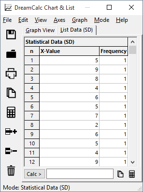
The most convenient method of data input is to use the spreadsheet style interface provided in the Graphing & List Window. The main calculator interface is instantly aware of any modifications you make here.
Keying in List Data
You can use the Edit menu to insert and remove list rows, and sort data according to the selected column.
If you are working with the SD list, the Consolidate Frequencies option will sort the list and combine any cells which share the same value by summing their frequencies. Whereas the Edit→Prune option will simply remove empty cells, or cells containing invalid data.
If you only have a few data points, you can use the calculator keypad to add values to the list in sequence.
To enter a value, simply key it in and press [DAT]. You should use the separator key [;] to enter paired values, for example:
45 [;] 3
[DAT]
In Statistical Data (SD) mode, this will enter a value of 45 with a frequency of 3, or an X-Y pair in a regression mode. If you omit the frequency in SD mode, a value of 1 will be assumed.
To clear the list from the keypad, click [CLRMEM] and select "Stats".
There are two ways to perform statistical calculations, as follows.
Statistical calculations are possible from the list page-tab of the Graphing & List Window.
Simply select from the Calc button to perform a calculation.
On the main keypad, you will find the following statistical keys:
These keys allow input of statistical functions using an on-screen menu selection. You can page through the available functions by pressing the respective key repeatedly.
The following examples demonstrate calculation from the keypad using prefix algebraic input order. If you are using postfix algebraic or RPN, you must adjust the example input to suit.
Bring up the Graphing & List Window by pressing F12 and switch to the list page. Ensure that calculator is in SD mode by selecting the option Mode→Standard Data from the list window's menu.
Key in (or copy and paste) the following 44 sample measurements into the SD list. All frequencies should be 1.
10.88 10.25 10.2 8.71 11.23 10.88 12.33 10.67 9.96 9.08 8.76 |
9.23 10.56 11.09 10.7 11.08 9.84 9.59 8.22 9.89 10.6 10.61 |
9.12 9.6 10.58 9.11 10.02 10.51 10.96 11.11 9.85 8.95 10.16 |
10.11 9.39 9.28 10.27 9.52 9.1 10.1 9.65 8.48 9.47 10 |
Sample Measurement Values
Example 1: Mean & Confidence Interval.
Calculate an estimate of the mean based upon the above sample, and estimate a confidence interval (CI) for a 90% confidence level.
From the calculator keypad, key in:
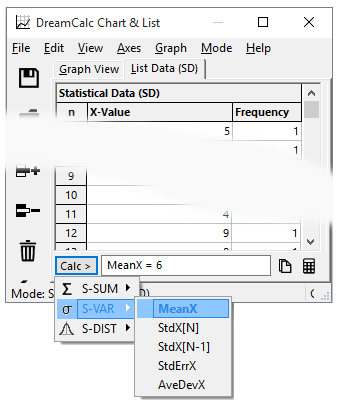
[S-VAR] and select MeanX
Displays: 9.99318181818181818 (mean)
Alternatively, you can use the Calc button menu from the list window, as shown in the screen-shot above.
Now, the CI of the mean is given by the equation:
CI = t * StdErr
where t is the two-sided Student t-value normally found by reference to statistical tables. However, since we have more than 30 measurements, we will use DreamCalc's standard z-score function in place of the t-value, as follows:
[zs] (z-score function above the [;] key)
0.9 (90% confidence as fraction)
[×]
[S-VAR] and select StdErrX
[ENTER]
Displays: 0.21161705529476782 (CI)
Therefore, the mean is 9.9931 +/- 0.2116 with a 90% level of confidence.
Example 2: Observation Probability.
Assuming that the above data is normally distributed with a true mean of 10, estimate the probability of observing a measurement outside the range 8.8 to 11.2.
To solve this, we could calculate the normalized variate of the lower value 8.8. and then use the DreamCalc PG function to give the probability of observing a value smaller than 8.8. Because we know that the distribution is normal, thus symmetrical, we can simply multiply by 2 give the probability of a observing a value on either side of the stated range.
Key in the following to perform this:
[PG] (probability from -INF to z)
[S-DIST] and select Z
8.8
[×]
2
[ENTER]
Displays: 0.162068
Put the calculator into cubic regression mode and copy the following data into the X-Y list.
Speed mph (X) 10 20 30 40 50 60 70 80 |
Fuel Economy mpg (Y) 22 42 46 48 45 41 39 38 |
Sample "Fuel Economy" Data
Import File: sample_xy_data.txt
Example 1: Regression Coefficients.
Calculate the coefficients A, B, C and D, for a line of best fit where: y = Ax3 + Bx2 + Cx + D.
[S-DIST] and select COEF_A
Displays: 4.31818181818181818E-4

[S-DIST] and select COEF_B
Displays: -0.07168831168831169

[S-DIST] and select COEF_C
Displays: 3.52326839826840218

[S-DIST] and select COEF_D
Displays: -5.5714285714292907
Example 2: Calculate Y as Function of X.
Estimate the fuel economy at 15 mph. Also estimate an error for the result.
We can use the FofX function to give y (fuel economy) as a function of x (speed), as follows:
[S-DIST] and select FofX
15
[ENTER]
Displays: 32.6051136363629757 (estimated fuel economy)
Furthermore, we can use the RMSE (root mean square error) to give the average error from the regression line:
[S-DIST] and select RMSE
Displays: 1.26659261574385245 (estimated error)
NOTE. Press [S-DIST] twice if RMSE is not visible.
Therefore, we can say the fuel economy at 15 mph is 32.6 +/- 1.3 (approx.).
DreamCalc Graphing and Professional Edition users will be able to produce the plot below using the Graphing & List Window.
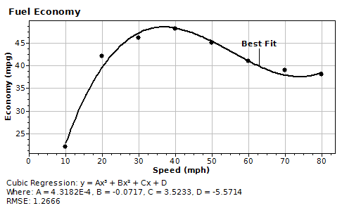
If the above chart is not visible, select Graph→X-Y Data Charts→Scatter Points from the Graphing & List Window menu.
See also: Statistical Functions, Statistical Data Charts, Logistic Regression