

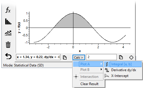
The Calc button provides numerical calculus options
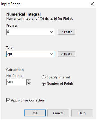
Integral parameters dialog window
Numerical integrals, derivatives (dy/dx) and x-axis intercepts can be found for any X-Y plot using the Calc button at the bottom of the Graphing & List Window. Additionally, the intersection points of dual function plots can be determined.
To calculate the area under a curve, select the integral option using the Calc button, and input the required x value range as prompted (see below right). The integral can be found for both function plots and X-Y list plots.
The "Apply Error Correction" option adjusts the final value, and rounds it to a number of digits applicable to its accuracy. Generally, this option should be checked.
When the option is unchecked, however, the result is calculated without adjustment and shown along with its estimated error — the estimated difference between it and the true value. For example, with the option unchecked, an example result output would be:
8.18512216971 (E=-0.00169)
When checked, the example result above would be displayed simply as: 8.18.
The origin and significance of the error term is described in the following section.
DreamCalc uses the composite trapezoidal rule to calculate the integral as follows:
T(f) ≈ 0.5 × Σ (xk+1 - xk) ( f(xk+1) + f(xk) ) [k=1, N-1] (eq. 1)
Where T(f) is the integral of function f(x) numerically calculated using N number of points (thus N-1 trapezoids).
The error involved in this numerical calculation is given by:
E(f) = - (xN - x1)³ × f''(ξ) / 12(N-1)² (eq. 2)
Refer: https://en.wikipedia.org/wiki/Trapezoidal_rule
Note that the above source writes N for the number of intervals, rather than points.
This value represents the difference between the result as estimated by eq. 1, and the true result of the integration. Here, ξ respresents some [unknown] value within the integral range. By summing the error terms for each trapazoid individually (i.e. we make N=2, and sum the individual results over N-1 instead), we can write:
E(f) = - Σ (xk+1 - xk)³ × f''(ξk) / 12 [k=1, N-1] (eq. 3)
Now the value ξk is some point between xk and xk+1 for each interval. In this next step, we assume that ξk lies at the midway point of each interval, or:
ξk ≈ 0.5 × (xk+1 + xk) (eq. 4)
Finally, given no knowledge of the "true integral", we can nevertheless estimate the error term as follows:
E(f) ≈ - Σ (xk+1 - xk)³ × f''(0.5 × (xk+1 + xk)) / 12 [k=1, N-1] (eq. 5)
Therefore, we can generally improve on the accuracy of eq. 1 by adding the above estimated error to yield a "corrected" result:
Tc(f) ≈ T(f) + E(f) (eq. 6)
To summarize, checking the "Apply Error Correction" option gives the result Tc(f), whereas leaving it unchecked gives T(f) and E(f) seperately.
In this example, we integrate the following function over the range [1, 6] for a number of numerical steps:
f(x) = 2 + sin(2 * √x) (eq. 7)
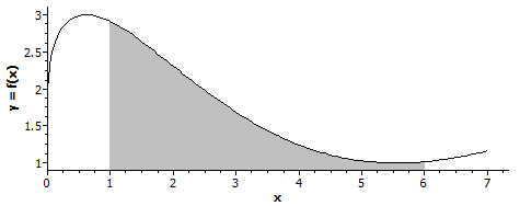
For this equation, we know that the true value for the integral over [1, 6] is 8.1834792077. Therefore, using the results below, we can see how accuracy is improved as we decrease the interval h by increasing the number of steps N.
| No. Intervals | Steps N | h | T(f) | E(f) estimate* | E(f) true* | Tc(f, h) |
|---|---|---|---|---|---|---|
| 10 | 11 | 0.5 | 8.19385456517 | -0.0117 | -0.01037535747 | 8.2 |
| 25 | 26 | 0.2 | 8.18512216971 | -0.00169 | -0.00164296201 | 8.18 |
| 50 | 51 | 0.1 | 8.18388931918 | -4.14E-4 | -4.1011148E-4 | 8.184 |
| 100 | 101 | 0.05 | 8.18358169603 | -1.03E-4 | -1.0248833E-4 | 8.184 |
| 500 | 501 | 0.01 | 8.18348330669 | -4.1E-6 | -4.09899E-6 | 8.18348 |
* The estimated error is given by eq. 5, whereas the true error can by found by: E(f) = 8.1834792077 - T(f).
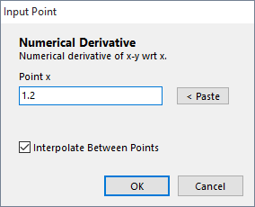
To calculate the gradient of a curve at a specified point, select the derivative option using the Calc button, and input the required x value as prompted. The gradient can be calculated for both function and list data plots provided the specified point is within the graphed range.
For this, function graphing should already be selected, i.e. Graph→Function Graph.
The symmetric difference quotient technique is used to calculate the derivate with respect to x according to the following:
f'(x) = [ f(x+h) - f(x-h) ] / 2h (eq. 8)
Where h is an interval automatically chosen as follows:
h = 1E-7 |x| (eq. 9)
For x ≠ 0. Where x = 0, h = 1E-7 is used.
In other words, the accuracy of the result is independent of the plotting interval used to generate the curve, and the final result will be shown rounded to an estimated number of digits of accuracy.
To calculate the gradient at a point within a list of X-Y values, the graphing window must be set to show an X-Y data plot, rather than the function grapher. For example, select the Graph→X-Y Data Plots→Line Plot menu option.
In calculating the result, an interpolation technique may optionally be used, as selected by the "Interpolate Between Points" option in the input window (see right). This improves accuracy provided the data points represent spot values on a smoothly varying trend, rather than descrete discontinuities.
When interpolation is used, the result will be rounded to an estimated number of digits of accuracy. If "Interpolate Between Points" is unselected, however, the result will simply be the gradient of the straight-line formed between the two data points adjacent to the input x value, and rounded to 12 decimal places.
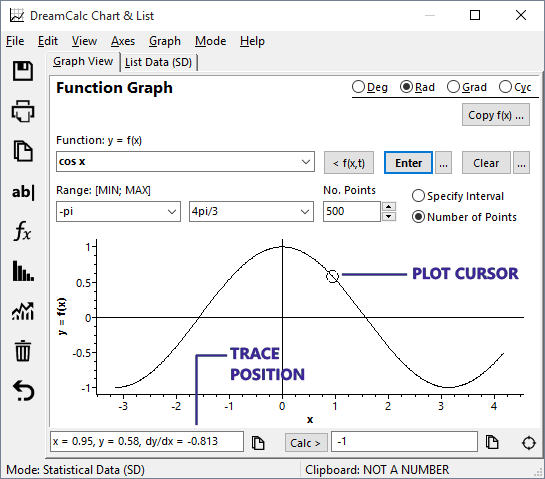
The cursor position and gradient (see below right) are shown beneath the chart. You will see this update as you move the cursor over a plot. The gradient is calculated using the line connecting the two points either side of the cursor position, and should be treated as an approximate value only. You can use the Calc button to find more accurate results.
You can find x-axis intercepts for any plot, and points of intersection where two function plots are displayed on the same graph. If there is more than one intersection between the plots, you will be prompted for which point to find. In this case, input "1" for the first point, or "2" for the second etc.
The result will be displayed to an estimated number of digits of accuracy. The accuracy will be determined by the number of plotted data points, and where there are few data points and potential accuracy is low, an indication will be shown to signify the approximate nature of the result.
Notes. Intersection points are determined using a numerical method which cannot usually find intersections where the area of intersection is zero.
See also: Graphing a Function, and Graphing Examples.